Posts tagged "study":
KAIST CS431 Notes
Notes for KAIST CS431: Concurrent Programming.
Lecture videos are here.
Some topics may be out of the course scope, but come up along this note-taking process.
1. thread::scope
fn increment_both_half(data: &mut [i32]) {
    let (left, right) = data.split_at_mut(data.len() / 2);

    thread::scope(|scope| {
        scope.spawn(|_| {
            for x in left {
                *x += 1;
            }
        });

        scope.spawn(|_| {
            for x in right {
                *x += 1;
            }
        });
    });

    println!(date);
}
- Use
thread::scopewhen the threads must borrow data owned by the current stack frame. Otherwise`thread::spawn` would fail as it requires'staticor clone. - The
Scopeis only returned when all threads are joined (and consequently blocks), ensuring threads cannot outlive the borrowed data
2. unsafe fn
pub struct NonZeroUsize(usize);

pub fn make_nonzero(x: usize) -> Option<NonZeroUsize> {
    if x == 0 {
        None
    } else {
        Some(NonZeroUsize(x))
    }
}

pub unsafe fn consume_nonzero(x: u32) -> NonZeroUsize {
    NonZeroUsize(x)
}
- Mark a function as
unsafewhen calling it requires the caller to upload some invariants which the compiler cannot guarantee. - Whether a function is
unsafehas nothing to do with its implementation, e.g., the API can be safe with unsafe code block. - Calling an
unsafe fnmust be wrapped withunsafe {}block.
3. object safety
- Object safety is a set of rules whether a trait can be used for dynamic dispatch, i.e.,
dyn trait. - These rules are already listed in 2024-12-28-interesting-rust-snippets.html.
- These rules ensure
- A sized
vtablecan be built for each concrete implementation of the trait (rule 1), and - The caller can know the type size returned from any trait method call (rule 2).
- A sized
4. async_trait
trait Data {
    fn fetch(&self) -> Pin<Box<dyn Future<Output = String> + Send>>;
}

// is equivalent to

#[async_trait]
trait Data {
    async fn fetch(&self) -> String;
}
async_traitis only necessary for dynamic dispatch. For static dispatch, one can just writeasync fn fetch() -> String.- Why
Box<dyn Future>notimpl Future: to know type size during compiler time. Why
Pin: to prevent the future being moved and self-reference is broken when the future changes state, e.g.,async fn fetch(&self) { let data = String::from("hello"); let reference = &data; // reference to local variable is stored as absolute address some_async().await; // suspend here println!("{}", reference); // resume here, reference still needed }
CS110L Notes
Notes for CS110L Safety in Systems Programming. Mostly follow Spring 2020, also include Spring 2021.
Not complete, only started taking notes since Lec 10 (2020).
1. Channel
- Golang: Do not communicate by sharing memory; instead, share memory by communicating.
- Message passing: each thread has its own memory, they communicate only by message exchanging.
- In theory, this implies: no shared memory -> no data races -> each thread needs to copy the data -> expensive
- In practice, goroutines share heap memory and only make shallow copies into channels -> pass pointers to channel is dangerous!
- In Rust, passing pointers, e.g.,
Boxis always safe due to ownership transfer - An ideal channel: MPMC (multi-producer, multi-consumer).
1.1. Mutex-based channel implementation
pub struct SemaPlusPlus<T> {
    queue_and_cv: Arc<(Mutex<VecDeque<T>>, Condvar)>,
}

impl<T> SemaPlusPlus<T> {
    pub fn send(&self, message: T) {
        let (queue_lock, cv) = &*self.queue_and_cv;
        let mut queue = queue_lock.lock().unwrap();
        let queue_was_empty = queue.is_empty();
        queue.push_back(message);
        // if a queue is not empty, then another thread must have notified and main()
        // must be awake
        if queue_was_empty {
            cv.notify_all();
        }
    }

    pub fn recv(&self) -> T {
        let (queue_lock, cv) = &*self.queue_and_cv;
        // wait_while dereferences the guard and pass the protected data to the closure,
        // when the condition is true, it releases the lock and sleep until another thread
        // notify_all
        let mut queue = cv
            .wait_while(queue_lock.lock().unwrap(), |queue| queue.is_empty())
            .unwrap();
        queue.pop_front().unwrap()
    }
}

fn main() {
    let sem: SemaPlusPlus<String> = SemaPlusPlus::new();
    let mut handlers = Vec::new();
    for i in 0..NUM_THREADS {
        let sem_clone = sem.clone();
        let handle = thread::spawn(move || {
            rand_sleep();
            sem_clone.send(format!("thread {} just finished!", i))
        });
        handlers.push(handle);
    }
    // main is the only consumer of the queue,
    // it wakes up when some thread notify_all, locks the queue, consume the message
    // and release the lock until it is notified again
    for _ in 0..NUM_THREADS {
        println!("{}", sem.recv())
    }

    for handle in handlers {
        handle.join().unwrap();
    }
}
- Mutex-based channel is inefficient:
- it does not allow the queue producer and consumer modify the queue simultaneously.
- It involves system calls.
- Go channels are MPMC, but it essentially implement
Mutex<VecDeque<>>with fuxtex.
1.2. Rust crossbeam channel implementation
- Minimal lock usage.
- Channels are not the best choice for global values -> lock still required.
/// Factor the number while receiving numbers from stdin
fn main() {
    let (sender, receiver) = crossbeam_channel::unbounded();
    let mut threads = Vec::new();
    for _ in 0..num_cpus::get() {
        // The channel maintains a reference counter for senders and for receivers
        // when receiver.clone(), the receiver counter increments.
        let receiver = receiver.clone();
        threads.push(thread::spawn(move || {
            while let Ok(next_num) = receiver.recv() {
                factor_number(next_num);
            }
        }));
    }

    let stdin = std::io::stdin();
    for line in stdin.lock().lines() {
        let num = line.unwrap().parse::<u32>().unwrap();
        sender.send(num).expect("Cannot send to channel when there is no receiver");
    }

    // decrement the sender counter, when no sender, the channel is closed
    drop(sender);

    for thread in threads {
        thread.join().expect("panic");
    }
}
2. Networking systems
2.1. System
2.1.1. File system
- Open file (OF) table: system-wide table, stores file position, access mode (read/write) and reference count.
- File descriptor (FD) table: process-specific table, maps file descriptor integers to references in the OF table; multiple FD entries can point to the same OF entry (e.g., parent and child processes share file positions).
- Vnode table: system-wide table, contains file (e.g., terminal, socket) size, permissions, timestamps, disk block locations; multiple OF entries can reference the same vnode entry, indicating same file opened multiple times.
2.1.2. Start a server
- A process creates a socket file descriptor with a queue for connection requests.
- The process binds the socket with specific IP and port.
- The process listens and accepts connections in a loop.
2.1.3. Connect to a server (ignore networking details)
- The client creates a socket and send the socket address in the SYN packet.
- The server accpets the request and start a new clinet-specific socket to establish a bidirectional communication channel.
2.2. Scalability and avilability
- Internet traffic has grown faster than hardware has increased in power.
- Two machines with commodity performance is much cheaper than one machine with 2x performance.
- Need to distribute a system’s functionality over servers using networking.
- Scale out: separate stateless computation and data storage.
- Chaos engineering: intentionally introduce failures on production, e.g., randomly terminates an entire datacenter or even a region.
2.2.1. Load balancers
- Relay client requests to one compute node; health check each compute node.
- Load balancing load balancers:
- Round-robin DNS; DNS return multiple IPs for the same hostname.
- Hard to consistently rotate IPs if the DNS responses are cached.
- DNS has no idea of IP health.
- Geographic routing: DNS servers respond with the load balancer IP closest to the client.
- If the cloest data center is done, availability is still broken.
- IP anycast: multiple computers announce they own the same IP (BGP).
- Round-robin DNS; DNS return multiple IPs for the same hostname.
2.3. Security
- Authentication: who are you? Authorization: are you allowed?
- Prevent confidential data leakage: use a framework to handle every request, check authenticartion/authorization; use type systems.
- Elasticsearch: distributed, open source search and analytics engine for all types of data; involved in multiple data breach incidents.
- Why: bad default settings, e.g., default username and password; accept all connections by default.
- Design principles: needs to be harder to do things wrong than to do thing right.
3. Event-driven programming
- Threads: a lightweight process; has own stack, CPU registers, status; managed by OS scheduler, e.g., swap on and off the core.
- States: block, ready, running
- Block syscalls: every thread runs for a time slice before switched by OS, or give up the slice early if it is blocked by e.g.,
read,waitpid,cv.wait,lock,sleep. - Switching threads are expensive:
- Context switching cost: switch virtual address space, restore register and cache, etc.
- Memory overhead: each thread consumes stack memory.
- The thread could have done other work when it is blocked on one request.
- Non-blocking I/O: One thread handles concurrent I/O with Epoll, which repeatedly notifies what file descriptors are ready for I/O.
- Key problem: state management.
3.1. Rust future
- Fututres are single eventual values produced by asynchronous computations.
- Keep track of in-progress operations along with associated state; each future handles one operation.
/// A simplified version of Future definition
trait Future {
type Output;
// the executor thread calls poll() to start running until it cannot progress
// cx includes a wake() function so that the future wakes up the executor when it can progress again
// when wake() is called, the executor uses cx to identify the future that can make new progress
fn poll(&mut self, cx: &mut Context) -> Poll<Self::Output>;
}

enum Poll<T> {
Ready(T),
/// Allow the single thread to work on other future
Pending,
}
- In practice, futures are composed with various combinators.
// This is just an example to show combinator,
// it is not real code, as this is hard to maintain when complexity increases
// and shared data must be propogated through the chain even if they are not always used
fn addToInbox(email_id: u64, recipient_id: u64) -> impl Future<Output = Result<(), Error>> {  // return type is tedious
    loadMessage(email_id)
        // message is needed in get_recipient, but later future needs
        .and_then(|message| get_recipient(message, recipient_id))
        .map(|(message, recipient)| recipient.verifyHasSpace(&message))
        .and_then(|(message, recipient)| recipient.addToInbox(message))
}
- Can write futures that depend on multiple concurrently-executing futures.
let cook_meal_future = futures::future::join(
    vec![
        CookMeatFuture::new(),
        CookMeatFuture::new(),
        // future may return Pending after complete 2 futures,
        // the next time when the executor calls poll(), the state is restored
        CookSoupFuture::new(),
        BakeBreadFuture::new()
    ]
);
- Syntax suger:
asyncandawait.
// An async function is a function that returns future
// the compiler transform the code into Future with poll()
async fn addToInbox(email_id: u64, recipient_id: u64) -> Result<(), Error> {
    // .await waits for a future and gets its value
    let message = loadMessage(email_id).await?;
    let recipient = get_recipient(recipient_id).await?;
    recipient.verifyHasSpace(&message)?;  // this is a normal function
    recipient.addToInbox(message).await
}
- An async function does not do anything when running it, its purpose is to produce a future that does the stuff written in the function.
3.1.1. Executor
- An executor loops over futures that can currently make progress and call
pollon them; or go to sleep until some future callswake. - A popular executor is Tokio; it allows multiple executors to execute futures in parallel.
- Need to protect shared data with synchronization primitives acorss futures.
- Futures cannot block, e.g., call
lock, otherwise the executor cannot continue other futures.- Tokio provides a non-blocking versions for synchronization primitives.
3.1.2. Tokio
- Convert blocking functions into async versions.
use tokio::io::{AsyncReadExt, AsyncWriteExt};
use tokio::net::TcpListener;  // should not block in async code

// futures do not do anything until an executor executes them
// the macro generates a sync main which creates a runtime executor
// and submits the returned future to the executor
#[tokio::main]
async fn main() {
let listener = TcpListener::bind("127.0.0.1:8080").await.unwrap();
loop {
    let (mut socket, _) = listener.accept().await.unwrap();
    tokio::spawn(async move {  // an async block
        let mut buf = [0; 1024];
        let n = socket.read(&mut buf).await.unwrap();
        socket.write_all(&buf[0..n]).await.unwrap();
    });
}
}
3.1.3. Compilation
- Normal (synchronous) code stores variables on the stack.
- When calling another function, the inner function gets a new stack frame and CPU remembers the return address.
- When the function returns, the stack frame is popped and CPU jumps back to the return address.
- Async functions may return multiple times at each
.await, everytime it returns, the stack frame is popped, so the async function needs to maintain its state in its returned future object. - The compiler transforms the async function into a state enum that implements
Futureand an implementation ofpoll().
enum AddToInboxState {
    NotYetStarted {
        email_id: u64,
        recipient_id: u64,
    },
    WaitingLoadMessage {
        recipient_id: u64, // the data is to be used in the next state
        state: LoadMessageFuture,
    },
    WaitingGetRecipient {
        message: Message,
        state: GetRecipientFuture,
    },
    WaitingAddToInbox {
        state: AddToInboxFuture,
    },
    Completed {
        result: Result<(), Error>,
    },
}

// this is only concept code, not real implementation
fn poll() {
    match self.state {
        NotYetStarted(email_id, recipient_id) => {
            let next_future = load_message(email_id);
            self.state = AddToInboxState::WaitingLoadMessage {
                recipient_id: *recipient_id,
                state: next_future,
            };
        }
        WaitingLoadMessage(recipient_id, state) => {
            match state.poll() {
                Ready(message) => {
                    let next_future = get_recipient(recipient_id);
                    // switch to WaitingGetRecipient state
                }
                Pending => return Pending,
            }
        }
        WaitingGetRecipient(message, state) => {
            match state.poll() {
                Ready(recipient) => {
                    recipient.verifyHasSpace(&message)?;
                    let next_future = recipient.addToInbox(message);
                    // switch to WaitingAddToInbox state
                }
                Pending => return Pending,
            }
        }
    }
}
- All compiled futures are registered in the executor, the executor works as a scheduler and polls each future when it wakes up.
- The executor does not care each future’s internal state, this is maintained in the future context.
- The executor polls
mainfuture first and run until it reaches.await. - When an async function polls another async function, if the inner future returns
Pending, the outer future also returnsPending; when the inner future is ready, it wakes the whole task in the executor, and the executor polls outer future again. - Sync functions consume stack, async functions consume heap as each future is live on heap.
- Usage: I/O bound and highly concurrent, e.g., thousand network connections, DB queries.
C++ feature introduction
This is a personal not for the CMU 15-445 C++ bootcamp along with some explanation from Claude.ai.
1. Namespace
- Provides scopes to identifiers with
::. Namespaces can be nested.
#include <iostream>
namespace ABC {
    void spam(int a) { std::cout << "Hello from ABC::spam" << std::endl; }
    // declare a nested namespace
    namespace DEF {
    void bar(float a) { std::cout << "Hello from ABC::DEF::bar" << std::endl; }
    void use_spam(int a) {
    ABC::spam(a);
    // no difference with ABC::spam(a) if DEF
    // does not have a spam function
    spam(a);
    }
} // namespace DEF

    void use_DEF_bar(float a) {
    // if a namespace outside of DEF wants to use DEF::bar
    // it must use the full namespace path ABC::DEF::bar
    DEF::bar(a);
    }

} // namespace ABC
- Two namespaces can define functions with the same name and signatures.
- Name resolution rules: first check in the current scope, then enclosing scopes, finally going outward until it reaches the global scope.
- Can use
using namespace Bto use identifiers inBin the current scope without specifyingB::, this is not a good practice. - Can also only bring certain members of a namespace into the current scope, e.g.,
using C::eggs.
2. Wrapper class
Used to manage a resource, e.g., memory, file sockets, network connections.
class IntPtrManager {
private:
  // manages an int* to access the dynamic memory
  int *ptr_;
};
- Use the RAII (Resource Acquisition is Initialization) idea: tie the lifetime of a resource to the lifetime of an object.
- Goal: ensure resources are released even if an exception occurs.
Acquisition: resources are acquired in the constructor.
class IntPtrManager {
public:
  // the constructor initializes a resource
  IntPtrManager() {
    ptr_ = new int;  // allocate the memory
    *ptr_ = 0;  // set the default value
  }

  // the second constructor takes an initial value
  IntPtrManager(int val) {
    ptr_ = new int;
    *ptr_ = val;
  }
};
Release: resources are released in the destructor.
class IntPtrManager {
public:
  ~IntPtrManager() {
    // ptr_ may be null after the move
    // don't delete a null pointer
    if (ptr_) {
      delete ptr_;
    }
  }
};
A wrapper class should not be copyable to avoid double deletion of the same resource in two destructors.
class IntPtrManager {
public:
  // delete copy constructor
  IntPtrManager(const IntPtrManager &) = delete;
  // delete copy assignment operator
  IntPtrManager &operator=(const IntPtrManager &) = delete;
};
A wrapper class is still moveable from different lvalues/owners.
class IntPtrManager {
public:
  // a move constructor
  // called by IntPtrManager b(std::move(a))
  IntPtrManager(IntPtrManager &&other) {
    // while other is a rvalue reference, other.ptr_ is a lvalue
    // therefore a copy happens here, not a move
    // in the constructor this.ptr_ has not pointed to anything
    // so no need to delete ptr_
    ptr = other.ptr_;
    other.ptr_ = nullptr;  // other.ptr_ becomes invalud
  }

  // move assignment operator
  // this function is used by c = std::move(b) operation
  // note that calling std::move() does not require implementing this operator
  IntPtrManager &operator=(IntPtrManager &&other) {
    // a self assignment should not delete its ptr_
    if (ptr_ == other.ptr_) {
      return *this;
    }
    if (ptr_) {
      delete ptr_; // release old resource to avoid leak
    }
    ptr_ = other.ptr_;
    other.ptr_ = nullptr;  // invalidate other.ptr_
    return *this;
  }
};
3. Iterator
Iterators, e.g., pointers, are objects that point to an element inside a container.
int *array = malloc(sizeof(int) * 10);
int *iter = array;
int zero_elem = *iter;
// use ++ to iterate through the C style array
iter++;
// deference the operator to return the value at the iterator
int first_elem = *iter;
- Two main components of an iterator:
- Dereference operator
*: return the value of the element of the current iterator position. - Increment
++: increment the iterator’s position by 1- Postfix
iter++: return the iterator before the increment (Iterator). - Prefix
++iter: return the result of the increment (Iterator&). ++iteris more efficient.
- Postfix
- Dereference operator
- Often used to access and modify elements in C++ STL containers.
3.1. A doubly linked list (DLL) iterator
Define a link node:
struct Node {
  // member initializer list, e.g., next_(nullptr) equals to next_ = nullptr
  Node(int val) : next_(nullptr), prev_(nullptr), value_(val) {}

  Node *next_;
  Node *prev_;
  int value_;
};
Define the iterator for the DLL:
class DLLIterator {
public:
  // takes in a node to mark the start of the iteration
  DLLIterator(Node *head) : curr_(head) {}

  // prefix increment operator (++iter)
  DLLIterator &operator++() {
    // must use -> to access the member of a pointer!
    // use . if accessing the object itself
    curr_ = curr_->next_;
    return *this;
  }

  // postfix increment operator (iter++)
  // the (int) is a dummy parameter to differentiate
  // the prefix and postfix increment
  DLLIterator operator++(int) {
    DLLIterator temp = *this;
    // this is a pointer to the current object
    // *this returns the iterator object
    // ++*this calls the prefix increment operator,
    // which equals to `this->operator++()`
    ++*this;
    return temp;
  }

  // implement the equality operator
  // an lvalue reference argument avoids the copy
  // the const in the parameter means this function
  // cannot modify the argument
  // the `const` outside the parameter list means
  // the function cannot modify `this`
  bool operator==(const DLLIterator &str) const {
    return itr.curr_ == this->curr_;
  }

  // implement the dereference operator to return the value
  // at the current iterator position
  int operator*() { return curr_->value_; }

private:
  Node *curr_;
};
Define DLL:
class DLL {
public:
  DLL() : head_(nullptr), size_(0) {}

  // the destructor deletes nodes one by one
  ~DLL() {
    Node *current = head_;
    while (current != nullptr) {
      Node *next = current->next_;
      delete current;
      current = next;
    }
    head_ = nullptr;
  }

  // after the insertion `new_node` becomes the new head
  // `head` is just a pointer to the node
  void InsertAtHead(int val) {
    Node *new_node = new Node(val);
    // new_node->next points to the object pointed by head_
    new_node->next_ = head_;

    if (head_ != nullptr) {
      head_->prev_ = new_node;
    }

    head_ = new_node;
    size_ += 1;
  }

  DLLIterator Begin() { return DLLIterator(head_); }

  // returns the pointer pointing one after the last element
  // used in the loop to determine whether the iteration ends
  // e.g., `for (DLLIterator iter = dll.Begin(); iter != dll.End(); ++iter)`
  DLLIterator End() { return DLLIterator(nullptr); }

  Node *head_{nullptr};  // in-class initializers
  size_t size_;
};
4. STL containers
- The C++ STL (standard library) is a generic collection of data structure and algorithm implementations, e.g., stacks, queues, hash tables.
- Each container has own header, e.g.,
std::vector. - The
std::setis implemented as a red-black tree.
4.1. Vector
#include <algorithm> // to use std::remove_if
#include <iostream>  // to use std::cout
#include <vector>
// A helper class used for vector
class Point {
public:
  // constructors
  Point() : x_(0), y_(0) {}
  Point(int x, int y) : x_(x), y_(y) {}
  // inline asks the compiler to substitute the function
  // directly at the calling location instead of performing
  // a normal function call, to improve performance for small functions
  inline int GetX() const { return x_; }
  inline void SetX(int x) { x_ = x; }

  void PrintPoint() const {
    std::cout << "Point: (" << x_ << ", " << "y_" << ")\n";
  }

private:
  int x_;
  int y_;
};

int main() {
  std::vector<Point> point_vector;
  // approach 1 to append to a vector
  point_vector.push_back(Point(35, 36));
  // approach 2, pass the argument to Point(x,y) constructor
  // slightly faster than push_back
  point_vector.emplace_back(37, 38);
  // iterate through index
  // size_t: unsigned integers specifially used in loop or counting
  for (size_t i = 0; i < point_vector.size(); ++i) {
    point_vector[i].PrintPoint();
  }
  // iterate through mutable reference
  for (Point &item : point_vector) {
    item.SetX(10);
  }
  // iterate through immutable reference
  for (const Point &item : point_vector) {
    item.GetX();
  }

  // initialize the vector with an initializer list
  std::vector<int> int_vector = {0, 1, 2, 3};
  // erase element given its index
  // int_vector.begin() returns a std::vector<int>::iterator
  // pointing to the first elemnt in the vector
  // the vector iterator has a plus iterator
  int_vector.erase(int_vector.begin() + 2); // {0, 1, 3}
  // erase a range of elements
  // int_vector.end() points to the end of a vector (not the last element)
  // and cannot be accessed.
  int_vector.erase(int_vector.begin() + 1, int_vector.end()); // {0}
  // erase elements via filtering
  // std::remove_if(range_begin, range_end, condition) returns an iterator
  // pointing to the first element to be erased
  // remove_if() also partitions point_vector so that unsatisfied elements are
  // moved before the point_vector.begin(), i.e., the vector is reordered
  point_vector.erase(
      std::remove_if(point_vector.begin(), point_vector.end(),
                     [](const Point &point) { return point.GetX() == 10; }),
      point_vector.end());

  return 0;
}
4.2. Set
#include <iostream>
#include <set>

int main() {
  std::set<int> int_set;
  // can insert element with .insert() or .emplace()
  // .emplace() allows to construct the object in place
  for (int i = 1; i <= 5; ++i) {
    int_set.insert(i);
  }
  for (int i = 6; i <= 10; ++i) {
    int_set.emplace(i);
  }
  // iterate the set
  for (std::set<int>::iterator it = int_set.begin(); it != int_set.end();
       ++it) {
    std::cout << *it << " ";
  }
  std::cout << "\n";
  // .find(key) returns an iterator pointing to the key
  // if it is in the set, otherwise returns .end()
  std::set<int>::iterator search = int_set.find(2);
  if (search != int_set.end()) {
    std::cout << "2 is not found\n";
  }
  // check whether the set contains a key with .count()
  // it returns either 0 or 1 as each key is unique
  if (int_set.count(11) == 0) {
    std::cout << "11 is not in the set.\n";
  }
  // erase a key, returns the count of removed elements 0 or 1
  int_set.erase(4);
  // erase a key given its position, returns the iterator to the next element
  int_set.erase(int_set.begin());
  // erase a range of elements
  int_set.erase(int_set.find(9), int_set.end());
}
4.3. Unordered maps
#include <iostream>
#include <string>
#include <unordered_map>
#include <utility> // to use std::make_pair

int main() {
  std::unordered_map<std::string, int> map;
  // insert items
  map.insert({"foo", 2});
  map.insert({{"bar", 1}, {"eggs", 2}});
  // insert items via pairs
  map.insert(std::make_pair("hello", 10));
  // insert items in an array-style
  map["world"] = 3;
  // update the value
  map["foo"] = 9;
  // .find() returns an iterator pointing to the item
  // or the end
  std::unordered_map<std::string, int>::iterator result = map.find("bar");
  if (result != map.end()) {
    // one way to access the item
    // both '\n' and std::endl prints newliine, but std::endl
    // also flushes the output buffer, so use '\n' is better
    std::cout << "key: " << result->first << " value: " << result->second
              << std::endl;
    // another way is dereferencing
    std::pair<std::string, int> pair = *result;
    std::cout << "key: " << pair.first << " value: " << pair.second
              << std::endl;
    // check whether a key exists with .count()
    if (map.count("foo") == 0) {
      std::cout << "foo does not exist\n";
    }
    // erase an item via a key
    map.erase("world");
    // or via an iterator
    map.erase(map.find("bar"));
    // can iterate the map via iterator or via for-each
    for (std::unordered_map<std::string, int>::iterator it = map.begin();
         it != map.end(); ++it) {
      std::cout << "(" << it->first << ", " << it->second << "), ";
    }
    std::cout << "\n";
  }
}
5. auto
autokeyword tells the compiler to infer the type via its initialization expression.
#include <vector>
#include<unordered_map>
#include<string>
#include<iostream>
// create very long class and function
template <typename T, typename U> class VeryLongTemplateClass {
public:
  VeryLongTemplateClass(T instance1, U instance2)
      : instance1_(instance1), instance2_(instance2) {}

private:
  T instance1_;
  U instance2_;
};

template <typename T> VeryLongTemplateClass<T, T> construct_obj(T instance) {
  return VeryLongTemplateClass<T, T>(instance, instance);
}

int main() {
  auto a = 1;                        // a is int
  auto obj1 = construct_obj<int>(2); // can infer
  // auto defaults to copy objects rather than taking the reference
  std::vector<int> int_values = {1, 2, 3, 4};
  // a deep-copy happens
  auto copy_int_values = int_values;
  // this creates a reference
  auto &ref_int_values = int_values;
  // use auto in the for loop is very common
  std::unordered_map<std::string, int> map;
  for (auto it = map.begin(); it != map.end(); ++it) {
  }
  // another exmaple
  std::vector<int> vec = {1, 2, 3, 4};
  for (const auto &elem : vec) {
    std::cout << elem << " ";
  }
  std::cout << std::endl;
}
6. Smart pointers
- A smart pointer is a data structure used in languages that do not have built-in memory management (e.g., with garbage collection, e.g., Python, Java) to handle memory allocation and deallocation.
std::unique_ptrandstd::shared_ptrare two C++ standard library smart pointers, they are wrapper classes over raw pointers.std::unique_ptrretains sole ownership of an object, i.e., no two instances ofunique_ptrcan manage the same object, aunique_ptrcannot be copied.std::shared_ptrretains shared ownership of an object, i.e., multiple shared pointers can own the same object and can be copied.
6.1. std::unique_ptr
#include <iostream>
#include <memory>  // to use std::unique_ptr
#include <utility> // to use std::move

// class Point is the same as before

// takes in a unique point reference and changes its x value
void SetXTo10(std::unique_ptr<Point> &ptr) { ptr->SetX(10); }
int main() {
  // initialize an empty unique pointer
  std::unique_ptr<Point> u1;
  // initialize a unique pointer with constructors
  std::unique_ptr<Point> u2 = std::make_unique<Point>();
  std::unique_ptr<Point> u3 = std::make_unique<Point>(2, 3);
  // can treat a unique pointer as a boolean to determine whether
  // the pointer contains data
  std::cout << "Pointer u1 is " << (u1 ? "not empty" : "empty") << std::endl;
  if (u2) {
    std::cout << u2->GetX() << std::endl;
  }
  // unique_ptr has no copy constructor!
  std::unique_ptr<Point> u4 = u3; // won't compile!
  // can transfer ownership with std::move
  std::unique_ptr<Point> u5 = std::move(u3); // then u3 becomes empty!
  // pass the pointer as a reference so the ownership does not change
  SetXTo10(u5); // can still access u5 afterwards
  return 0;
}
- Note that the compiler does not prevent 2 unique pointers from pointing to the same object.
// the following code can compile
// but it causes a double deletion!
MyClass *obj = new MyClass();
std::unique_ptr<MyClass> ptr1(obj);
std::unique_ptr<MyClass> ptr2(obj);
6.2. std::shared_ptr
#include <iostream>
#include <memory>
#include <utility>

// class Point is the same as before

// modify a Point inside a shared_ptr by passing the reference
void modify_ptr_via_ref(std::shared_ptr<Point> &point) { point->SetX(10); }
// modify a Point inside a shared_ptr by passing the rvalue reference
// If an object is passed by rvalue reference, one should assume the ownership
// is moved after the function call, so the original object cannot be used
void modify_ptr_via_rvalue_ref(std::shared_ptr<Point> &&point) {
  point->SetY(11);
}
// copy a shared_pointer with the default constructor
// so one should define own copy constructor and assignment when an object
// contains pointers
void copy_shard_ptr_in_function(std::shared_ptr<Point> point) {
  std::cout << "Use count of the shared pointer: " << point.use_count()
            << std::endl; // add by 1
  // the copy is destroyed at the end, so the count is decremented
}

int main() {
  // the pointer constructors are the same as unique_ptr
  std::shared_ptr<Point> s1;
  std::shared_ptr<Point> s2 = std::make_shared<Point>();
  std::shared_ptr<Point> s3 = std::make_shared<Point>(2, 3);
  // copy a shared pointer via copy assignment or copy constructor
  // increment the reference count, which can be tracked by .use_count
  std::cout << "Use count of s3" << s3.use_count() << std::endl; // 1
  std::shared_ptr<Point> s4 = s3; // copy assignment
  std::cout << "Use count of s3" << s3.use_count() << std::endl; // 2
  std::shared_ptr<Point> s5(s4);
  std::cout << "Use count of s3" << s3.use_count() << std::endl; // 3
  s3->SetX(100); // also changes the data in s4 and s5
  std::shared_ptr<Point> s6 = std::move(s5); // s5 transfer the ownership to s6
  std::cout << "Use count of s3" << s3.use_count()
            << std::endl; // still 3: s3, s4, s6
  // as unique_ptr, shared_ptr can be passed by references and rvalue references
  modify_ptr_via_ref(s2);                   // setX(11)
  modify_ptr_via_rvalue_ref(std::move(s2)); // setY(12)
  std::cout << "s2.x = " << s2->GetX()
            << " , s2.y = " << s2->GetY(); // (11, 12)
  // shared_ptr can also be passed by value/copy
  std::cout << "Use count of s2" << s2.use_count() << std::endl; // 1
  copy_shared_ptr_in_function(s2); // inside the function, the use count is 2
  std::cout << "Use count of s2" << s2.use_count()
            << std::endl; // 1 again as the copy is detroyed
  return 0;
}
7. Synchronization
7.1. std::mutex
#include <iostream>
#include <mutex>
#include <thread>

// define a global variable to be modified
// by multiple threads
int count = 0;
// declare a mutex
std::mutex m;
void add_count() {
  m.lock(); // acquire the lock
  count += 1;
  m.unlock(); // release the lock
}
int main() {
  std::thread t1(add_count);
  std::thread t2(add_count);
  t1.join();
  t2.join();
  std::cout << count << std::endl; // always 2
  return 0;
}
7.2. std::scoped_lock
- A mutex wrapper that provides a RAII-style of obtaining and releasing the lock.
- When the object is constructed, the locks are acquired; when the object is destructured, the locks are released.
- Better than
std::mutexsince it provides exception safety.
#include <iostream>
#include <mutex>

int count = 0;
std::mutex m;
void add_count() {
  // the scoped_lock constructor allows for the thread
  // to acquire the mutex m
  std::scoped_lock slk(m);
  count += 1;
  // once the function finishes, slk is destructurd and
  // m is released
}
7.3. std::condition_variable
- Allow threads to wait until a particular condition before acquiring a mutex.
- Allow other threads to signal waiting threads to alert them that the condition may be true.
notify_one
#include <condition_variable>
#include <iostream>
#include <mutex>
#include <thread>

int count = 0;
std::mutex m;
// declare a condition variable
std::condition_variable cv;
void add_count_and_notify() {
  std::scoped_lock slk(m);
  count += 1;
  if (count == 2) {
    // notidy one waiting thread
    // otherwise the waiter thread hangs forever
    cv.notify_one();
  }
}
void waiter_thread() {
  // a unique_lock is movable but not copiable
  // more flexible than scoped_lock as it can unlock
  // and relock manually, while scoped_lock can only be
  // unlocked automatically.
  // scoped_lock cannot be used with condition variables
  std::unique_lock lk(m);
  cv.wait(lk, [] { return count == 2; });
  std::cout << count << std::endl;
}
int main() {
  std::thread t1(waiter_thread);
  // make t1 really waits
  std::this_thread::sleep_for(std::chrono::milliseconds(100));
  std::thread t2(add_count_and_notify);
  std::thread t3(add_count_and_notify);
  t1.join();
  t2.join();
  t3.join();
  return 0;
}
7.4. Reader-writer lock
- A reader-writer lock allows multiple threads to have shared read access (no writers are allowed during read operations) and exclusive write access, i.e., no other readers or writers are allowed during the write.
- C++ does not have a specific reader-writer’s lock library, but can be emulated with
std::shared_mutex,std::shared_lockandstd::unique_lock. std::shared_mutexis a mutex that allows for both shared read-only locking and exclusive write-only locking.std::shared_lockcan be used as an RAII-style read lock.std::unique_lockcan be used a RAII-style exclusive write lock.#include <iostream> #include <mutex> #include <shared_mutex> #include <thread> int count = 0; // resource std::shared_mutex m; void read_value() { // use shared_lock to gain read-only, shared access std::shared_lock lk(m); std::cout << "Reading " + std::to_string(count) << std::endl; } void write_value() { // use unique_lock to gain exclusive access std::unique_lock lk(m); count += 3; } int main() { // since all 3 threads run in parallel, // the output is not deterministic std::thread t1(read_value); std::thread t2(write_value); std::thread t3(read_value); t1.join(); t2.join(); t3.join(); return 0; }
CMU 15-445 notes: Hash Tables
This is a personal note for the CMU 15-445 L7 notes as well as some explanation from Claude.ai.
1. DBMS data structure application
- Internal meta-data: page tables, page directories.
- Tuple storage on disk.
- Table indices: easy to find specific tuples.
1.1. Design decisions
- Data layout for efficient access.
- Concurrent access to data structures.
2. Hash tables
- Implements an associative array that maps keys to values.
- On average \(O(1)\) operation complexity with the worst case \(O(n)\); \(O(n)\) storage complexity.
- Optimization for constant complexity is important in real world.
2.1. Where are hash tables used
- For tuple indexing. While tuples are stored on pages with NSM or DSM, during the query the DBMS needs to quickly locate the page that stores specific tuples. It can achieve this with separately-stored hash tables, where each key can be a hash of a tuple id, and the value points the location.
3. Hash function
- Maps a large key space into a smaller domain.
- Takes in any key as input, and returns a deterministic integer representation.
- Needs to consider the trade-off between fast execution and collision rate.
- Does not need to be cryptographically.
- The state-of-art (Fall 2023) hash function is XXHash3.
4. Hashing scheme
- Handles key collision after hashing.
- Needs to consider the trade-off between large table allocation (to avoid collision) and additional instruction execution when a collision occurs.
5. Static hashing scheme
- The hash table size is fixed; the DBMS has to rebuild a larger hash table (e.g., twice the size) from scratch when it runs out of space.
5.1. Linear probe hashing
- Insertion: when a collision occurs, linearly search the adjacent slots in a circular buffer until a open one is found.
- Lookup: search linearly from the first hashed slot until the desired entry or an empty slot is reached, or every slot has been iterated.
- Requires to store both key and value in the slot.
- Deletion: simply deleting the entry prevents future lookups as it becomes empty; two solutions:
- Replace the deleted entry with a dummy entry to tell future lookups to keep scanning.
- Shift the adjacent entries which were originally shifted, i.e., those who were originally hashed to the same key.
- Very expensive and rarely implemented in practice.
- The state-of-art linear probe hashing is Google
absl::flat_hash_map.
5.1.1. Non-unique keys
- The same key may be associated with multiple different values.
- Separate linked list: each value is a pointer to a linked list of all values, which may overflow to multiple pages.
- Redundant keys: store the same key multiple times with different values.
- A more common approach.
- Linear probing still works, if it is fine to get one value.
5.1.2. Optimization
- Specialized hash table based on key types and size; e.g., for long string keys, one can store the pointer or the hash of the long string in the hash table.
- Store metadata in a separate array, e.g., store empty slot in a bitmap to avoid looking up deleted keys.
- Version control of hash tables: invalidate entries by incrementing the version counter rather than explicitly marking the deletion.
5.2. Cuckoo hashing
- Maintains multiple hash tables with different hash functions to generate different hashes for the same key using different seeds.
- Insertion: check each table and choose one with a free slot; if none table has free slot, choose and evict an old entry and find it another table.
- If a rare cycle happens, rebuild all hash tables with new seeds or with larger tables.
- \(O(1)\) lookups and deletion (also needs to store keys), but insertion is more expensive.
- Practical implementation maps a key to different slots in a single hash table.
6. Dynamic hashing schemes
- Resize the hash table on demand without rebuilding the entire table.
6.1. Chained Hashing
- Maintains a linked list of buckets for each slot in the hash table; keys hashed to the same slot are inserted into the linked list.
- Lookup: hash to the key’s bucket and scan for it.
- Optimization: store bloom filter in the bucket pointer list to tell if a key exist in the linked list.
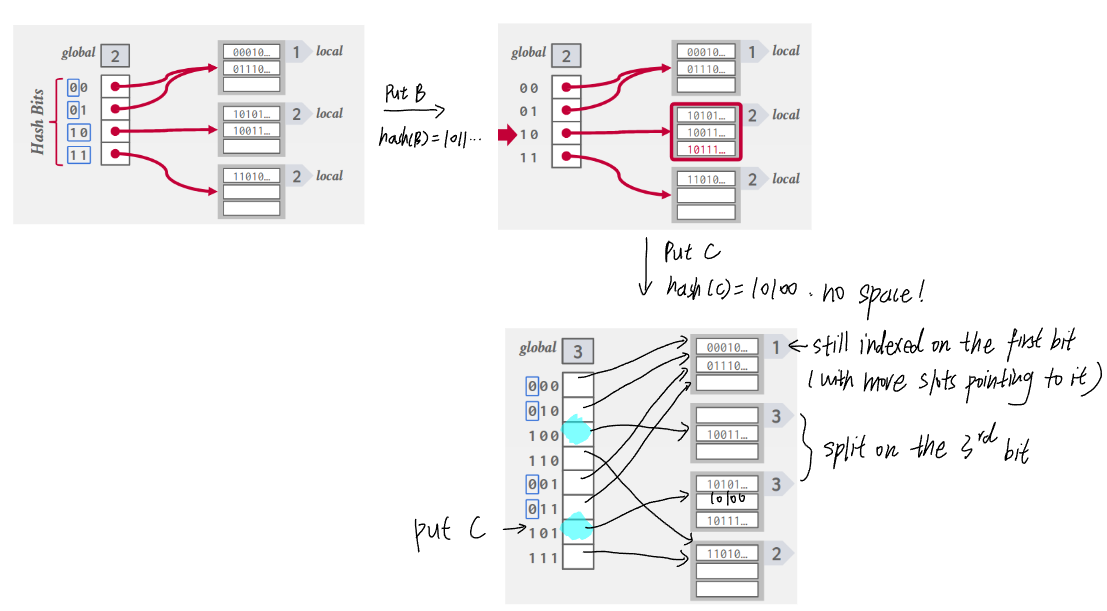
6.2. Extendible hashing
- Improve chained hashing to avoid letting chains grow forever.
- Allow multiple slot locations in the hash table to point to the same chain.
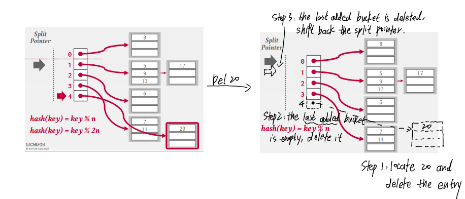
6.3. Linear hashing
- Maintains a split pointer to keep track of next bucket to split, even if the pointed bucket is not overflowed.
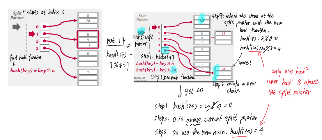
- There are always only 2 hash functions: \((key\ mod\ n)\) and \((key\ mod\ 2n)\) where \(n\) is the length of buckets when the split pointer is at the index 0 (i.e., the bucket length at any time is \(n + index(sp)\)).
- Why does \(k\ mod\ 2n < n + sp\) hold?
- A key is only mod by \(2n\) if the result of \((k\ mod\ n)\) is above the split pointer, i.e., \(0 \leq k\ mod\ n < sp)\).
- Let \(r = k\ mod\ n\), then \(k = pn + r\) and \(0 \leq r < sp\).
- Let \(r' = k\ mod\ 2n\), then \(k = q(2n) + r'\).
- If \(p = 2m\), then we also have \(k = m(2n) + r = q(2n) + r'\), in this case \(0 \leq r = r' < sp\).
- If \(p = 2m + 1\), then we have \(k = m(2n) + r + n = q(2n) + r'\), in this case \(n \leq r' = n + r < n + sp\).
CMU 15-445 notes: Memory Management
This is a personal note for the CMU 15-445 L6 notes as well as some explanation from Claude.ai.
1. Goals
- Manage DBMS memory and move data between the memory and the disk, such that the execution engine does no worry about the data fetching.
- Spatial control: keep relevant pages physically together on disk.
- Temporal control: minimize the number of stalls to read data from the disk.
2. Locks & Latches
- Both used to protect internal elements.
2.1. Locks
- A high-level logical primitive to allow for transaction atomicity.
- Exposed to users when queries are run.
- Need to be able to rollback changes.
2.2. Latches
- A low-level protection primitive a DBMS uses in its internal data structures, e.g., hash tables.
- Only held when the operation is being made, like a mutex.
- Do not need to expose to users or used to rollback changes.
3. Buffer pool
- An in-memory cache of pages read from the disk.
- The buffer pool’s region of memory is organized as an array of fixed size pages; each array entry is called a frame.
- When the DBMS requests a page, the buffer pool first searches its cache, if not found, it copies he page from the disk into one of its frame.
- Dirty pages (i.e., modified pages) are buffered rather than writing back immediately.
3.1. Metadata
- Page table: An in-memory hash mapping page ids to frame locations in the buffer pool.
- Dirty flag: set by a thread whenever it modifies a page to indicate the pages must be written back to disk.
- Pin/Reference counter: tracks the number of threads that are currently accessing the page; the storage manager is not allowed to evict a page if its pin count is greater than 0.
3.2. Memory allocation policies
- The buffer pool decides when to allocate a frame for a page.
- Global policies: decisions based on the overall workload, e.g., least recently used (LRU) or clock algorithm.
- Local policies: decisions applying to specific query, e.g., priority-based page replacement.
4. Buffer pool optimizations
4.1. Multiple buffer pools
- Each database or page can have its own buffer pool and adopts local policies to reduce latch contention.
- To map a page to a buffer pool, the DBMS can use object IDs or page IDs as the key.
- Record ID: a unique identifier for a row in a table (cf. Tuple layout post).
- Object ID: a unique identifier for an object, used to reference a user-defined type.
4.2. Pre-fetching
- While the first set of pages is being processed, the DBMS can pre-fetch the second set into the buffer pool based on the dependency between pages.
- E.g., If pages are index-organized, the sibling pages can be pre-fetched.
4.3. Scan sharing
- Query cursors can reuse retrieved data.
- When a query comes while a previous query is being processed by scanning the table, the new query can attach its scanning cursor to the first query’s cursor.
- The DBMS keeps track of where the second query joined to make sure it also completes the scan.
4.4. Buffer pool bypass
- Scanned pages do not have to be stored in the buffer pool to avoid the overhead.
- Use cases: a query needs to read a large sequence of contiguous pages; temporary pages like sorting or joins.
5. Buffer replacement policies
- The DBMS decides which page to evict from the buffer pool to free up a frame.
5.1. Least recently used (LRU)
- LRU maintains a timestamp of when each page was last accessed, and evicts the page with the oldest timestamp.
- The timestamp can be stored in a queue for efficient sorting.
- Susceptible to sequential flooding, where the buffer pool is corrupted due to a sequential scan.
- With the LRU policy the oldest pages are evicted, but they are more likely to be scanned soon.
5.2. Clock
- An approximation of LRU but replace the timestamp with a reference bit which is set to 1 when a page is accessed.
- Regularly sweeping all pages, if a bit is set to 1, reset to 0; if a bit is 0, evict the page.
5.3. LRU-K
- Tracks the last K accessed timestamps to predict the next accessed time, hence avoid the sequential flooding issue.
5.3.1. MySQL approximate LRU-K
- Use a linked list with two entry points: “old” and “young”.
- The new pages are always inserted to the head of “old”.
- If a page in the “old” is accessed again, it is then inserted to the head of “young”.
5.4. Localization
- Instead of using a global replacement policy, the DBMS make eviction decisions based on each query.
- Pages brought in by one query are less likely to evict pages that are important for other ongoing queries.
- The DBMS can predicts more accurately which pages should stay or be evicted once the query is complete, so that the buffer pool is less polluted with less useful pages.
5.5. Priority hint
- Transactions tell the buffer pool where pages are important based on the context of each page.
5.6. Dirty pages
- Two ways to handle dirty pages in the buffer pool:
- Fast: only drop clean pages.
- Slow: write back dirty pages to ensure persistent change, and then evict them (if they will not be read again.).
- Can periodically walk through the page table and write back dirty pages in the background.
6. Other memory pools
- A DBMS also maintains other pools to store:
- query caches,
- logs,
- temporary tables, e.g., sorting, join,
- dictionary caches.
7. OS cache bypass
- Most DBMS use direct I/O (e.g., with
fsyncinstead offwrite) to bypass the OS cache to avoid redundant page copy and to manage eviction policies more intelligently (cf. Why not OS post).
8. I/O scheduling
- The DBMS maintains internal queue to track page read/write.
- The priority are determined by multi-facets, e.g., critical path task, SLAs.
CMU 15-445 notes: Storage Models & Compression
This is a personal note for the CMU 15-445 L5 notes.
1. Database workloads
1.1. OLTP (Online Transaction Processing)
- Characterized by fast, repetitive, simple queries that operator on a small amount of data, e.g., a user adds an item to its Amazon cart and pay.
- Usually more writes than read.
1.2. OLAP (Online Analytical Processing)
- Characterized by complex read queries on large data.
- E.g., compute the most popular item in a period.
1.3. HTAP (Hybrid)
- OLTP + OLAP.
2. Storage models
- Different ways to store tuples in pages.
2.1. N-ary Storage Model (NSM)
- Store all attributes for a single tuple contiguously in a single page, e.g., slotted pages.
- Pros: good for queries that need the entire tuple, e.g., OLTP.
- Cons: inefficient for scanning large data with a few attributes, e.g., OLAP.
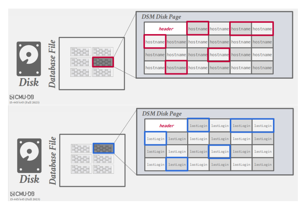
2.2. Decomposition Storage Model (DSM)
- Store each attribute for all tuples contiguously in a block of data, i.e., column store.
- Pros: save I/O; better data compression; ideal for bulk single attribute queries like OLAP.
- Cons: slow for point queries due to tuple splitting, e.g., OLTP.
- 2 common ways to put back tuples:
- Most common: use fixed-length offsets, e.g., the value in a given column belong to the same tuple as the value in another column at the same offset.
- Less common: use embedded tuple ids, e.g., each attribute is associated with the tuple id, and the DBMS stores a mapping to jump to any attribute with the given tuple id.
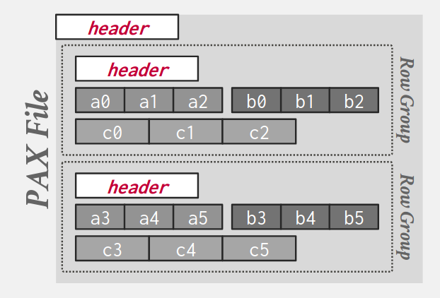
2.3. Partition Attributes Across (PAX)
- Rows are horizontally partitioned into groups of rows; each row group uses a column store.
- A PAX file has a global header containing a directory with each row group’s offset; each row group maintains its own header with content metadata.
3. Database compression
- Disk I/O is always the main bottleneck; read-only analytical workloads are popular; compression in advance allows for more I/O throughput.
- Real-world data sets have the following properties for compression:
- Highly skewed distributions for attribute values.
- High correlation between attributes of the same tuple, e.g., zip code to city.
- Requirements on the database compression:
- Fixed-length values to follow word-alignment; variable length data stored in separate mappings.
- Postpone decompression as long as possible during query execution, i.e., late materialization.
- Lossless; any lossy compression can only be performed at the application level.
3.1. Compression granularity
- Block level: compress all tuples for the same table.
- Tuple level: compress each tuple (NSM only).
- Attribute level: compress one or multiple values within one tuple.
- Columnar level: compress one or multiple columns across multiple tuples (DSM only).
3.2. Naive compression
- Engineers often use a general purpose compression algorithm with lower compression ratio in exchange for faster compression/decompression.
- E.g., compress disk pages by padding them to a power of 2KBs and storing them in the buffer pool.
- Why small chunk: must decompress before reading/writing the data every time, hence need o limit the compression scope.
- Does not consider the high-level data semantics, thus cannot utilize late materialization.
4. Columnar compression
- Works best with OLAP, may need additional support for writes.
4.1. Dictionary encoding
- The most common database compression scheme, support late materialization.
- Replace frequent value patterns with smaller codes, and use a dictionary to map codes to their original values.
- Need to support fast encoding and decoding, so hash function is impossible.
- Need to support order-preserving encodings, i.e., sorting codes in the same order as original values, to support range queries.
- E.g., when
SELECT DISTINCTwith pattern-matching, the DBMS only needs to scan the encoding dictionary (but withoutDISTINCTit still needs to scan the whole column).
- E.g., when
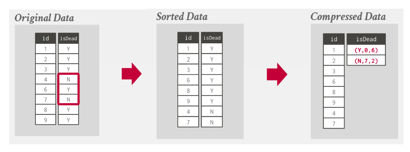
4.2. Run-Length encoding (RLE)
- Compress runs (consecutive instances) of the same value in a column into triplets
(value, offset, length). - Need to cluster same column values to maximize the compression.
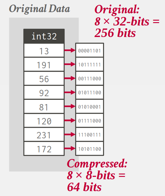
4.3. Bit-packing encoding
- Use less bits to store an attribute.
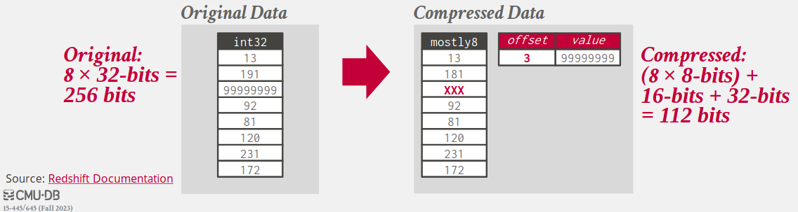
4.4. Mostly encoding
- Use a special marker to indicate values that exceed the bit size and maintains a look-up table to store them.
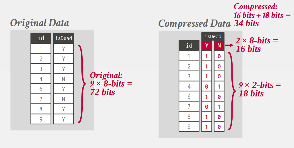
4.5. Bitmap (One-hot) encoding
- Only practical if the value cardinality is low.
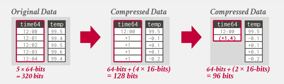
4.6. Delta encoding
- Record the difference between values; the base value can be stored in-line or in a separate look-up table.
- Can be combined with RLE encoding.
4.7. Incremental encoding
- Common prefixes or suffixes and their lengths are recorded to avoid duplication.
- Need to sort the data first.
CMU 15-445 notes: Database storage
This is a personal note for the CMU 15-445 L3 notes and CMU 15-445 L4 notes.
1. Data storage
1.1. Volatile device
- The data is lost once the power is off.
- Support fast random access with byte-addressable locations, i.e., can jump to any byte address and access the data.
- A.k.a memory, e.g., DRAM.
1.2. Non-volatile device
- The data is retained after the power is off.
- Block/Page addressable, i.e., in order to read a value at a particular offset, first need to load 4KB page into memory that holds the value.
- Perform better for sequential access, i.e., contiguous chunks.
- A.k.a disk, e.g., SSD (solid-state storage) and HDD (spinning hard drives).
1.3. Storage hierarchy
- Close to CPU: faster, smaller, more expensive.
1.4. Persistent memory
- As fast as DRAM, with the persistence of disk.
- Not in widespread production use.
- A.k.a, non-volatile memory.
1.5. NVM (non-volatile memory express)
- NAND flash drives that connect over an improved hardware interface to allow faster transfer.
2. DBMS architecture
- Primary storage location of the database is on disks.
- The DBMS is responsible for data movement between disk and memory with a buffer pool.
- The data is organized into pages by the storage manager; the first page is the directory page
- To execute the query, the execution engine asks the buffer pool for a page; the buffer pool brings the page to the memory, gives the execution engine the page pointer, and ensures the page is retained in the memory while being executed.
2.1. Why not OS
- The architecture is like virtual memory: a large address space and a place for the OS to bring the pages from the disk.
- The OS way to achieve virtual memory is to use
mmapto map the contents of a file in a process address space, and the OS is responsible for the data movement. - If
mmaphits a page fault, the process is blocked; however a DBMS should be able to still process other queries. - A DBMS knows more about the data being processed (the OS cannot decode the file contents) and can do better than OS.
- Can still use some OS operations:
madvise: tell the OS when DBMS is planning on reading some page.mlock: tell the OS to not swap ranges outs of disk.msync: tell the OS to flush memory ranges out to disk, i.e., write.
3. Database pages
- Usually fixed-sized blocks of data.
- Can contain different data types, e.g., tuples, indexes; data of different types are usually not mixed within the same page.
- Some DBMS requires each page is self-contained, i.e., a tuple does not point to another page.
- Each page is given a unique id, which can be mapped to the file path and offset to find the page.
3.1. Hardware page
- The storage that a device guarantees an atomic write, i.e., if the hardware page is 4KB and the DBMS tries to write 4KB to the disk, either all 4KB is written or none is.
- If the database page is larger than the hardware page, the DBMS requires extra measures to ensure the writing atomicity itself.
4. Database heap
- A heap file (e.g., a table) is an unordered collection of pages where tuples are stored in random order.
- To locate a page in a heap file, a DBMS can use either a linked list or a page directory.
- Linked list: the header page holds a pointer to a list of data and free pages; require a sequential scan when finding a specific page.
- Page directory: a DBMS uses special pages to track the location of each data page and the free space in database files.
- All changes to the page directory must be recorded on disk to allow the DBMS to find on restart.
5. Page layout
- Each page includes a header to record the page meta-data, e.g., page size, checksum, version.
- Two main approaches to laying out data in pages: slotted-pages and log-structured.
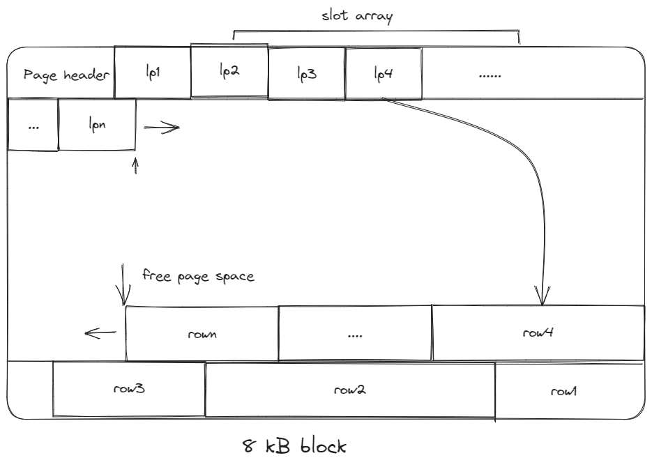
5.1. Slotted-pages
- The header keeps track of the number of used slots, the offset of the starting of each slot.
- When adding a tuple, the slot array grows from the beginning to the end, the tuple data grows from the end to the beginning; the page is full when they meet.
- Problems associated with this layout are:
- Fragmentation: tuple deletions leave gaps in the pages.
- Inefficient disk I/O: need to fetch the entire block to update a tuple; users could randomly jump to multiple different pages to update a tuple.
5.2. Log-structured
- Only allows creations of new pages and no overwrites.
- Stores the log records of changes to the tuples; the DBMS appends new log entries to an in-memory buffer without checking previous records -> fast writes.
- Potentially slow reads; can be optimized by bookkeeping the latest write of each tuple.
5.2.1. Log compaction
- Take only the most recent change for each tuple across several pages.
- There is only one entry for each tuple after the compaction, and can be easily sorted by id for faster lookup -> called Sorted String Table (SSTable).
- Universal compaction: any log files can be compacted.
- Level compaction: level 0 (smallest) files can be compacted to created a level 1 file.
- Write amplification issue: for each logical write, there could be multiple physical writes.
5.3. Index-organized storage
- Both page-oriented and log-structured storage rely on additional index to find a tuple since tables are inherently unsorted.
- In an index-organized storage scheme, the DBMS stores tuples as the value of an index data structure.
- E.g., In a B-tree indexed DBMS, the index (i.e., primary keys) are stored as the intermediate nodes, and the data is stored in the leaf nodes.
6. Tuple layout
- Tuple: a sequence of bytes for a DBMS to decode.
- Tuple header: contains tuple meta-data, e.g., visibility information (which transactions write the tuple).
- Tuple data: cannot exceed the size of a page.
- Unique id: usually page id + offset/slot; an application cannot rely on it to mean anything.
6.1. Denormalized tuple data
- If two tables are related, a DBMS can “pre-join” them so that the tables are on the same page.
- The read is faster since only one page is required to load, but the write is more expensive since a tuple needs more space (not free lunch in DB system!).
7. Data representation
- A data representation scheme specifies how a DBMS stores the bytes of a tuple.
- Tuples can be word-aligned via padding or attribute reordering to make sure the CPU can access a tuple without unexpected behavior.
- 5 high level data types stored in a tuple: integer, variable-precision numbers, fixed-point precision numbers, variable length values, dates/times.
7.1. Integers
- Fixed length, usually stored using the DBMS native C/C++ types.
- E.g.,
INTEGER.
7.2. Variable precision numbers
- Inexact, variable-precision numeric types; fast than arbitrary precision numbers.
- Could have rounding errors.
- E.g.,
REAL.
7.3. Fixed-point precision numbers
- Arbitrary precision data type stored in exact, variable-length binary representation (almost like a string) with additional meta-data (e.g., length, decimal position).
- E.g.,
DECIMAL.
7.4. Variable-length data
- Represent data of arbitrary length, usually stored with a header to keep the track of the length and the checksum.
- Overflowed data is stored on a special overflow page referenced by the tuple, the overflow page can also contain pointers to next overflow pages.
- Some DBMS allows to store files (e.g., photos) externally, but the DBMS cannot modify them.
- E.g.,
BLOB.
7.5. Dates/Times
- Usually represented as unit time, e.g., micro/milli-seconds.
- E.g.,
TIMESTAMP.
7.6. Null
- 3 common approaches to represent nulls:
- Most common: store a bitmap in a centralized header to specify which attributes are null.
- Designate a value, e.g.,
INT32_MIN. - Not recommended: store a flag per attribute to mark a value is null; may need more bits to ensure word alignment.
8. System catalogs
- A DBMS maintains an internal catalog table for the table meta-data, e.g., tables/columns, user permissions, table statistics.
- Bootstrapped by special code.
CMU 15-445 notes: Modern SQL
This is a personal note for the CMU 15-445 L2 notes, along with some SQL command explained by Claude.ai.
1. Terminology
1.1. SQL and relational algebra
- Relational algebra is based on sets (unordered, no duplicates); SQL is based on bags (unordered, allows duplicates).
- SQL is a declarative query language; users use SQL to specify the desired result, each DBMS determines the most efficient strategy to produce the answer.
1.2. SQL commands
- Data manipulation language (DML):
SELECT,INSERT,UPDATE,DELETE. Data definition language (DDL):
CREATE.CREATE TABLR student ( sid INT PRIMARY KEY, name VARCHAR(16), login VARCHAR(32) UNIQUE, age SMALLINT, gpa FLOAT );
- Data control language (DCL): security, access control.
2. SQL syntax
2.1. Join
Combine columns from one or more tables and produces a new table.
-- All students that get an A in 15-721
SELECT s.name
    FROM enrolled AS e, student AS s
WHERE e.grade = 'A' AND e.cid = '15-721'
    AND e.sid = s.sid
2.2. Aggregation function
AVG(COL),MIN(COL),MAX(COL),COUNT(COL).Take as input a bag of tuples and produce a single scalar value.
-- Get number of students and their average GPA with a '@cs' login
SELECT AVG(gpa), COUNT(sid) FROM student WHERE login LIKE '@cs';
-- Get the unique students
SELECT COUNT(DISTINCT login) FROM student WHERE login LIKE '@cs';
Non-aggregated values in
SELECToutput must appear inGROUP BY.-- Get the average GPA in each course SELECT AVG(s.gpa), e.cid FROM enrolled AS e, student AS s WHERE e.sid = s.sid GROUP BY e.cid;
HAVING: filter output results based on aggregation computation.SELECT AVG(s.gpa), e.cid FROM enrolled AS e, student AS s WHERE e.sid = s.sid GROUP BY e.cid HAVING AVG(s.gpa) > 3.9;
2.3. String operation
- Strings are case sensitive and single-quotes only in the SQL standard.
- Use
LIKEfor string pattern matching:%matches any sub-string,_matches any one character
- Standard string functions:
UPPER(S),SUBSTRING(S, B, E). ||: string concatenation.
2.4. Date and time
- Attributes:
DATE,TIME. - Different DBMS have different date/time operations.
2.5. Output redirection
One can store the results into another table
-- output to a non-existing table
SELECT DISTINCT cis INTO CourseIds FROM enrolled;
-- output to an existing table with the same number of columns and column type
-- but the names do not matter
INSERT INTO CourseIds (SELECT DISTINCT cid FROM enrolled);
2.6. Output control
- Use
ORDER,ASCandDESCto sort the output tuples; otherwise the output could have different order every time. Use
LIMIT,OFFSETto restrict the output number.SELECT sid FROM enrolled WHERE cid = '15-721' ORDER BY UPPER(grade) DESC, sid + 1 ASC; LIMIT 10 OFFSET 10; -- output 10 tuples, starting from the 11th tuple
2.7. Nested queries
- Nested queries are often difficult to optimize.
- The inner query can access attributes defined in the outer query.
Inner queries can appear anywhere.
-- Output a column 'one' with 1s, the number of 1s
-- equals to the number of rows in 'student'
SELECT (SELECT 1) AS one FROM student;

-- Get the names of students that are enrolled in '15-445'
SELECT name FROM students
    WHERE sid IN (
        SELECT sid FROM enrolled
        WHERE cid = '15-445'
);

-- Get student record with the highest id
-- that is enrolled in at least one course.
SELECT student.sid, name
    FROM student
    -- the intermediate output is aliases as max_e
    JOIN (SELECT MAX(sid) AS sid FROM enrolled) AS max_e
    -- only select student who has the max_e
    ON student.sid = max_e.sid;

-- the above is same as below, but `join` syntax is more preferred
SELECT student.sid, name
FROM student AS s, (SELECT MAX(sid) AS sid FROM enrolled) AS max_e
WHERE s.sid = max_e.sid;
- Nested query results expression:
ALL: must satisfy expression for all rows in sub-query.ANY,IN: must satisfy expression for at least one row in sub-query.EXISTS: at least one row is returned.-- Get all courses with no students enrolled in SELECT * FROM course WHERE NOT EXISTS( SELECT * FROM enrolled WHERE course.cid = enrolled.cid ) -- Get students whose gpa is larget than the highest score in '15-712' -- and the login has a level > 3 SELECT student.sid, name FROM student AS S WHERE s.gpa > ALL ( SELECT course.score FROM course WHERE course.cid = '15-712' ) AND student.login IN ( SELECT login FROM enrolled WHERE level > 3 );
2.8. Window functions
- Perform sliding calculation across a set of tuples.
2.9. Common Table Expressions (CTE)
- An alternative to windows or nested queries when writing more complex queries.
CTEs use
WITHto bind the output of an inner query to a temporary table.WITH cteName (col1, col2) AS ( SELECT 1, 2 ) SELECT col1 + col2 FROM cteName;
CMU 15-445 notes: Relational Model & Algebra
This is a personal note for the CMU 15-445 L1 video and CMU 15-445 L1 notes, along with some terminology explained by Claude.ai.
1. Terminology
1.1. Database
- An organized collection of inter-related data that models some aspect of the real-world.
1.2. Database design consideration
- Data integrity: protect invalid writing.
- Implementation: query complexity, concurrent query.
- Durability: replication, fault tolerance.
1.3. Database management system (DBMS)
- A software that manages a database.
- Allow the definition, creation, query, update and administration of databases.
1.4. Data model
- A conceptual, high-level representation of how data is structured
- Defines entities, attributes, relationships between entities and constraints.
1.5. Schema
- A concrete implementation of a data model.
- Defines tables, fields, data types, keys and rules.
- Typically represented by a specific database language.
1.6. Entities and Tables
- Entities: conceptual representations of objects in the logical data model.
- Tables: physical storage structures in the physical data model.
1.7. Attributes and Fields
- Attributes: properties of an entity.
- Fields: columns in a database table.
1.8. Logical layer
- The entities and attributes the database has.
1.9. Physical layer
- How are entities and attributes stored in the database.
1.10. Data manipulation languages (DMLs)
- Methods to store and retrieve information from a database.
- Procedural: the query specifies the (high-level) strategy the DBMS should use to get the results, e.g., with relational algebra.
- Declarative: the query specifies only what data is desired but not how to get it, e.g., with relational calculus (a formal language).
1.11. SQL (Structured Query Language) and relational model
- SQL implements the relational model in DBMS and provides a standard way to create, manipulate and query relational databases.
- Different SQL implementation may vary and do not strictly adhere to the relational model, e.g., allow duplicate rows.
2. Relational model
- A data model that defines a database abstraction to avoid maintenance overhead when changing the physical layer.
- Data is stored as relations/tables.
- Physical layer implementation and execution strategy depends on DBMS implementation.
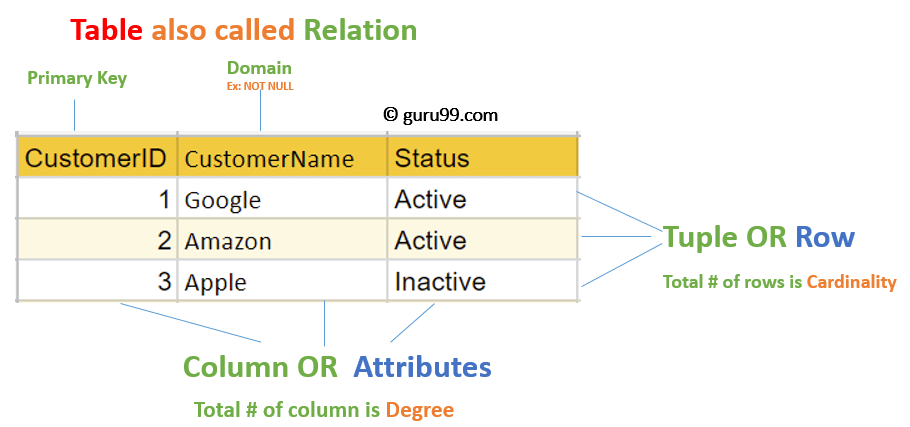
2.1. A relation
- An unordered set that contains the relationship of attributes that represent entities.
- Relationships are unordered in the relation.
2.2. A domain
- A named set of allowable values for a specific attribute.
2.3. A tuple
- A set of attribute values in the relation.
- Values can also be lists or nested data structures.
Null: a special value in any attribute which means the attribute in a tuple is undefined.- \(n-ary\): a relation with \(n\) attributes.
2.4. Keys
- Primary key: uniquely identifies a single tuple.
- Foreign key: specifies that an attribute (e.g.,
CustomerID) in one relation (e.g.,OrderTable) has to map to a tuple (e.g., the tuple with the sameCustomerID) in another relation (e.g.,CustomerTable).
3. Relational Algebra
- A set of fundamental operations to retrieve and manipulate tuples in a relation.
- Each operator takes in one or more relations as inputs, and outputs a new relation; operators can be chained.
- Is a procedure language, meaning the execution always follow the query, even there exists more efficient way to get the same result; A better way is to be more declarative, e.g., SQL’s
wheresyntax. - Common relational algebra.
Go patterns
This a personal note for the Russ Cox guest lecture.
1. Concurrency vs Parallelism
- Concurrency: write a program to handle lot of things at once
- not necessarily faster
- Parallelism: the program itself can do a lot of computations at once
2. Use goroutines for states
2.1. Matching a regex
- return if a given string matches a regex: start with
", contains arbitrary escape sequence and ends with" unclear logic: store states in the data
 1: state := 0
 2: for {
 3:     c := read()
 4:     switch state {
 5:     case 0:
 6:         // first char must be "
 7:         if c != '"' {
 8:             return false
 9:         }
10:         state = 1 // match the next char
11:     case 1:
12:         // ending with " matches
13:         if c == '"' {
14:             return true
15:         }
16:         if c == '\\' {
17:             state = 2
18:         } else {
19:             // transition to state 1 to match next char
20:             state = 1
21:         }
22:     case 2:
23:         // read the char, discard it and
24:         state = 1
25:     }
26: }
clear logic: store states in the code
 1: // no variable to store state
 2: if read() != '"' {
 3:     return false
 4: }
 5: var c rune // c is a Unicode, alias to int32
 6: for c != '"' {
 7:     c = read()
 8:     if c == '\\' {
 9:         read()  // skip the next char
10:     }
11: }
12: return true
2.2. When the state variable cannot be avoided
the function needs to return the state
 1: type quoter struct {
 2:     state int
 3: }
 4:
 5: func (q *quoter) Init() {
 6:     r.state = 0
 7: }
 8: // proess each char based on current state
 9: func (q *quoter) Write(c rune) Status {
10:     switch q.state {
11:     case 0:
12:         if c != '"' {
13:             return BadInput
14:         }
15:         q.state = 1
16:     case 1:
17:         if c == '"' {
18:             return Success
19:         }
20:         if c == '\\' {
21:             q.state = 2
22:         } else {
23:             q.state = 1
24:         }
25:     case 2:
26:         q.state = 1
27:     }
28:     return NeedMoreInput
29: }
use additional goroutines to hold states
1: type quoter struct { 2: char chan rune 3: status chan Status 4: } 5: func (q *quoter) Init() { 6: q.char = make(chan rune) 7: q.status = make(chan Status) 8: // need to make sure why and when the goroutine will exit 9: go q.parse() 10: // blocks until it receives an initial status from parse() 11: // to ensure that parse() is ready, i.e., q.status = NeedMoreInput 12: // before Write() is called 13: <-q.status 14: } 15: // Write sends the next char to q.char, which will be receivecd by parse() 16: // the status is a public state accessible by the user 17: func (q *quoter) Write(r rune) Status { 18: q.char <- c 19: // wait for the result 20: return <-q.status 21: } 22: func (q *quoteReader) parse() { 23: if q.read() != '"' { 24: q.status <- SyntaxError 25: return 26: } 27: var c rune 28: for c!= '"' { 29: c = q.read() 30: if c == '\\' { 31: q.read() 32: } 33: } 34: q.status <- Done 35: } 36: // a helper function used in parse() to return the next char in q.char 37: func (q *quoter) read() int { 38: q.status <- NeedMoreInput 39: return <- q.char 40: } 41: func main() { 42: q := "er{} 43: q.Init() 44: 45: input := `"Hello, \"World\""` 46: for _, c := range input { 47: status := q.Write(c) 48: } 49: }
- check goroutine blockage
Ctrl-\sendsSIGQUIT- use the HTTP server’s
/debug/pprof/goroutineif importingnet/http
3. Pattern 1: publish/subscribe server
- the information goes one way: server -> client
- close a channel to signal no new values will be sent
prefer
deferwhen unlocking the mutex1: type Server struct { 2: mu sync.Mutex // protect sub 3: sub map[chan<- Event]bool // whether a channel should be closed 4: } 5: func (s *Server) Init() { 6: s.sub = make(map[chan<- Event]bool) 7: } 8: // publish an event to all subscribed channel 9: func (s *Server) Publish(e Event) { 10: s.mu.Lock() // each method could be called by many clients 11: defer s.mu.Unlock() 12: // need mutex here since it needs to read s.sub state 13: for c := range s.sub { 14: // if a goroutine consumes the channel events too slow 15: // then a new event publish has to wait 16: // before it can send to the channel 17: // can add channel buffer to mitigate this 18: c <- e 19: } 20: } 21: // a channel starts to subscribe 22: func (s *Server) Subscribe(c chan<- Event) { 23: s.mu.Lock() 24: defer s.mu.Unlock() 25: if s.sub[c] { 26: // the mutex wil also be unlocked with defer 27: panic("pubsub: already subscribed") } 28: s.sub[c] = true 29: } 30: // a channel cancels the subscription 31: func (s *Server) Cancel(c chan<- Event) { 32: s.mu.Lock() 33: defer s.mu.Unlock() 34: if !s.sub[c] { 35: panic("pubsub: not subscribed") 36: } 37: close(c) 38: delete(s.sub, c) 39: }
3.1. Options for slow goroutines
- slow down event generation
- drop events if it cannot be sent, e.g.,
os/signal,runtime/pprof queue events, e.g., add a
helperbetween the server and each client, which also separates the concerns1: func helper(in <-chan Event, out chan<- Event) { 2: var q []Event 3: // if the in is closed, flash out the pending events in q 4: // and close out 5: for in != nil || len(q) > 0 { 6: // decide whether and what to send 7: var sendOut chan<- Event 8: var next Event 9: if len(q) > 0 { 10: sendOut = out 11: next = q[0] 12: } 13: select { 14: case e, ok := <-in: // never reaches here after in = nil 15: // ok tells whether in is closed 16: if !ok { 17: in = nil 18: break 19: } 20: q = append(q, e) 21: case sendOut <- next: // if len(q) == 0, sendOut = nil 22: q = q[1:] 23: } 24: } 25: close(out) 26: }
convert mutexes into goroutines, not suitable for Raft where state transition is complex
 1: type Server struct {
 2:     publish   chan Event
 3:     subscribe chan subReq  // a channel to queue unhandled subscription
 4:     cancel    chan subReq
 5: }
 6: type subReq struct {
 7:     c  chan<- Event
 8:     // a signal of whether an operation succeeds
 9:     ok chan bool
10: }
11:
12: func (s *Server) Init() {
13:     s.publish = make(chan Event)
14:     s.subscribe = make(chan subReq)
15:     s.cancel = make(chan subReq)
16:     go s.loop()
17: }
18: func (s *Server) Publish(e Event) {
19:     // no mutex is required here
20:     // as it does not read state
21:     s.publish <- e
22: }
23: func (s *Server) Subscribe(c chan<- Event) {
24:     r := subReq{c: c, ok: make(chan bool)}
25:     s.subscribe <- r
26:     if !<-r.ok {  // wait for loop() handle result
27:         panic("pubsub: already subscribed")
28:     }
29: }
30: func (s *Server) Cancel(c chan<- Event) {
31:     r := subReq{c: c, ok: make(chan bool)}
32:     s.cancel <- r
33:     if !<-r.ok {
34:         panic("pubusb: not subscribed")
35:     }
36: }
37: func (s *Server) loop() {
38:     // now sub is a local variable, no lock is needed
39:     // sub maps from a subscribed channel to a helper channel
40:     sub := make(map[chan<- Event]chan<- Event)
41:     for {
42:         select {
43:         case e := <-s.publish:
44:             for _, h := range sub {
45:                 // the event is published to a helper channel
46:                 h <- e
47:             }
48:         case r := <-s.subscribe:
49:             // the helper channel exists
50:             // meaning the subscriber has been handled before
51:             if sub[r.c] != nil {
52:                 r.ok <- false
53:                 break
54:             }
55:             h = make(chan Event)
56:             go helper(h, r.c)
57:             sub[r.c] = h
58:             r.ok <- true
59:         case c := <-s.cancel:
60:             if !sub[r.c] == nil{
61:                 r.ok <- false
62:                 break
63:             }
64:             // close the helper channel
65:             close(sub[r.c])
66:             delete(sub, r.c)
67:             r.ok <- true
68:         }
69:     }
70: }
4. Pattern 2: work scheduler
\(M\) tasks assigned to \(N\) servers/workers, \( M >> N\).
 1: func Schedule(servers []string, numTask int,
 2:     call func(srv string, task int)) {
 3:
 4:     idle := make(chan string, len(servers))
 5:     // initialize a channel of idle servers
 6:     for _, srv := range servers {
 7:         idle <- srv
 8:     }
 9:
10:     for task := 0, task < numTask; task++ {
11:         // if using task in the for loop rather than a local task,
12:         // there is a race: the loop goes on before the goroutinue starts,
13:         // so that some tasks are skipped.
14:         task := task
15:         // if moving srv := <- idle inside goroutine
16:         // a lot of goroutines are created simoutaneously and hung
17:         // due to non-idle server
18:         // leaving it outside so that a goroutine is only created when
19:         // there is an idle server (but it slows down the main loop)
20:         srv := <-idle
21:         go func() {
22:             call(srv, task) // server does the task
23:             // serve finishes the task and becomes idle again
24:             idle <- srv
25:         }()
26:     }
27:
28:     // determine when all tasks are done / all servers are idle
29:     // this is used to prevent early exit when all tasks have been assigned
30:     // but the last servers have not finished
31:     for i :=0; i < len(servers); i++ {
32:         <-idle
33:     }
34: }
Optimization for the above code: while the task loop creates goroutines \(M\) times, actually there are only at most \(N\) active goroutines at any time.
- Better to spin off a goroutine for each server.
- The number of servers can be dynamic.
 1: func Schedule(servers chan string, numTask int,
 2:     call func(srv string, task int)) {
 3:
 4:     work := make(chan int)  // a queue of all works yet to be done
 5:     done := make(chan bool) // a queue of all done tasks
 6:     exit := make(chan bool) // signal when should not pull new servers
 7:
 8:     runTasks := func(srv string) {
 9:         // keep polling until work is closed
10:         for task := range work {
11:             if call(srv, task) {
12:                 done <- true
13:             } else {
14:                 // repush the task if it failed
15:                 work <- task
16:             }
17:         }
18:     }
19:
20:     // use a goroutine to avoid hanging when
21:     // no server is available
22:     go func() {
23:         for _, srv := range servers {
24:             for {
25:                 select {
26:                 case src := <-servers:
27:                     go runTasks(srv)
28:                 case <-exit:
29:                     return
30:                 }
31:             }
32:         }
33:     }()
34:
35:     // The following code has a deadlock!
36:     // In the runTasks, the server pushes to done channel when a task is done.
37:     // However, the done channel is only pulled when the main routine has
38:     // pushed all tasks and close the work channel.
39:     // Therefore any server hangs when trying push the second done work.
40:     // for taks := 0; task < numTask; task++ {
41:     //  work <- task
42:     // }
43:     // // signal no more task so that servers know
44:     // // when to termiante
45:     // close(work)
46:
47:     // // wait until all tasks are done
48:     // for i := 0; i < numTask; i++ {
49:     //  <-done
50:     // }
51:
52:     // fix 1: one can switch between work and donw channel
53:     i := 0
54: WorkLoop:
55:     for task := 0; task < numTask; task++ {
56:         for {
57:             select {
58:             case work <- task:
59:                 continue WorkLoop
60:             case <-done:
61:                 i++
62:             }
63:         }
64:     }
65:
66:     // wait for the last assigned tasks to be done
67:     for ; i < numTask; i++ {
68:         <-done
69:     }
70:
71:     // only close work channel in the end,
72:     // in case some tasks failed and need to be redo
73:     close(work)
74:     exit <- true // stop pulling new servers
75:
76:     // fix 2: move the work assignment to a separate go routine
77:     // go func() {
78:     //  for task := ; task < numTask; task++ {
79:     //      work <- task
80:     //  }
81:     //  close(work)
82:     // }()
83:
84:     // fix 3: increase buffer for the work channel
85:     // work := make(chan int, numTask)
86: }
5. Pattern 3: replicated service client
A client replicates its requests to multiple servers, waits for the first reply and changes its preferred server.
func (c *Client) Call(args Args) Reply {
    type result struct {
        serverID int
        reply Reply
    }

    const timeout = 1 * time.Second
    t := time.NewTimer(timeout)
    defer t.Stop()

    // a channel for all servers to send reply
    // so that even if the client has received a reply
    // other later replies don't hang
    done := make(chan result, len(c.servers))

    c.mu.Lock()
    prefer := c.prefer
    c.mu.Unlock()

    var r result
    for off := 0; off < len(c.servers); off++ {
        // start from the preferred server
        id := (prefer + off) % len(c.servers)
        go func() {
            done <- result{id, c.callOne(c.servers[id], arfs)}
        }()

        // now wait for either a done signal or a timeout
        // if it is done, don't send to other servers
        // otherwise, reset the timer and sends to the next server
        select {
        case r = <-done:
            goto Done  // use a goto if it makes code clear
        case <-t.C:
            // timeout
            t.Reset(timeout)
        }
    }

    r = <-done  // wait for the first reply even if it is a RPC timeout

Done:
    c.mu.Lock()
    c.prefer = r.serverID // update preference
    c.mu.Unlock()
    return r.reply
}
6. Pattern 4: Protocol multiplexer
A multiplexer sits in front of a service and forward messages between multiple clients and the service, e.g., an RPC.
 1: type ProtocolMux interface {
 2:     // A mux is binded to a specific service
 3:     Init(Service)
 4:     // A client uses this method to send message to the service
 5:     // and wait for the service reply
 6:     Call(Msg) Msg
 7: }
 8:
 9: // Methods that a service exposes to let a mux use
10: // Underlining messgae processing are in the implementation
11: // of the actual service struct
12: type Service interface {
13:     // A tag is a muxing identifier in the request or reply message,
14:     // e.g., which client channel to send the reply
15:     ReadTag(Msg) int64
16:     // Send a request message to the service
17:     // multiple sends cannot be called concurrently
18:     // probably due to only a single channel between
19:     // mux and the service (serialization)
20:     Send(Msg)
21:     // Waits and return the reply message,
22:     // multiple recvs cannot be called concurrently
23:     Recv() Msg
24: }
The mux maintains a channel to queue unsent requests and a channel to queue unsent replies.
 1: type Mux struct {
 2:     srv Service
 3:     // stores unsent requests
 4:     send chan Msg
 5:     mu sync.Mutex
 6:     // maps channel tag to channel
 7:     // whose replies have not been sent out
 8:     pending map[int64]chan<- Msg
 9: }
10:
11: func (m *Mux) Init(srv Service) {
12:     m.srv = srv
13:     m.pending = make(map[int64]chan Msg)
14:     go m.sendLoop()
15:     go m.recvLoop()
16: }
17:
18: // sending out queued requests
19: func (m *Mux) sendLoop {
20:     for args := range m.send {
21:         m.srv.Send(args)
22:     }
23: }
24:
25: func (m *Mux) recvLoop() {
26:     for {
27:         reply := m.srv.Recv()
28:         tag := m.srv.ReadTag(reply)
29:         m.mu.Lock()
30:         // get the reply channel
31:         done := m.pending[tag]
32:         // clear the channel since the message loop
33:         // is complete
34:         delete(m.pending, tag)
35:         m.mu.Unlock()
36:
37:         if done == nil {
38:             panic("unexpected reply")
39:         }
40:         done <- reply
41:     }
42:
43: }
44:
45: // Clients call this method concurrently
46: func (m *Mux) Call(args Msg) (reply Msg) {
47:     tag := m.srv.ReadTag(args)
48:     // to record which message should reply
49:     // to which client
50:     done := make(chan Msg, 1)
51:     m.mu.Lock()
52:     if m.pending[tag] != nil {
53:         m.mu.Unlock()
54:         panic("duplicate request")
55:     }
56:     m.pending[tag] = done
57:     m.mu.Unlock()
58:     m.send <- args
59:     return <-done // hang until a reply is received
60: }
Weblab notes: React route
This is a personal note for the web.lab lectures.
1. Router
- use the Reach Reach Router library
URL -> Router -> render different components
1: <App>
2:   // conditional rendering based on curren url
3:   <Router>
4:     <Home path="/" /> // root path
5:     <Dashboard path="dashboard" /> // relative to the current URL
6:     <Team path="/team" /> // absolute path: root path + "/team"
7:     <NotFound default />
8:   </Router>
9: </App>;
2. Link
- relative:
<Link to="newpage">Click me</Link> - absolute:
<Link to="/newpage">Click me</Link>
3. Workshop 3
3.1. Structure
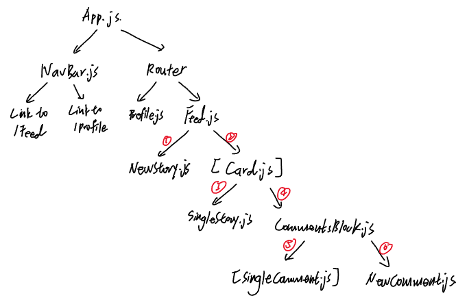
3.2. States
| name | states |
|---|---|
| Feed | stories: a list of stories |
| Card | comments: a list of comments for a story id |
3.3. Props
| index | props |
|---|---|
| 1 | a function to update stories |
| 2 | all attributes in a story |
| 3 | the attributes used to display a story |
| 4 | a story id; a list of comments under the story; a function to update comments |
| 5 | all attributes in a comment |
| 6 | a comment id; the function to update comments |
3.4. Why passing down the update function in props 1, 4, 6?
- To share the parent states, i.e.,
storiesandcommentsto child component. Since the post action happens in the child component, we need a way to automatically update the states to see new contents immediately.
Weblab notes: React hooks
This is a personal note for the web.lab lectures.
1. What is a React hook
- Special functions to access parts of the component lifestyle.
- e.g.,
useState
1.1. useState is not enough
1: const [persons, setPersons] = useState([]);
2:
3: testingStuff = () => {
4:     /* assume persons is empty before */
5:     setPersons([...persons, "me"]);
6: }
7: console.log(persons);
- The output of
console.logis[]instead of["me"]because setting a state is async! - To do something immediately after a state is changed, use
useEffecthook!
1.2. useEffect runs after specific variable change
1: useEffect(() => {
2:     console.log(persons);
3: }, [persons]);
1: useEffect(() => {
2: /* do something, e.g., interact with an external service */
3:
4: return () => {
5: /* cleanup function on dismount, e.g., disconnect from external service */
6: }
7: }, [/*dependencies */])
useEffect(myFunction, [var1, var2])callsmyFunctioneverytime whenvar1orvar2changesuseEffect(myFunction, []])calls only once when the component is rendered for the first time (on mount)useEffect(myFunction)calls at every render
2. React hook patterns
2.1. Fetch and send data
1: /* fetch data on mount */
2: useEffect(() => {
3:     get("/api/packages").then((packageList) => {
4:         setPackages(packageList);
5:     });
6: }, []);
1: /* send data then toggle admin state */
2: const handleToggleAdmin = () => {
3:     // .then(), do something once the promise is fulfilled
4:     post("/api/user/admin", { admin: !admin }).then(() => {
5:         setAdmin(!admin);
6:     });
7: };
8: /* <Button onClick={handleToggleAdmin} */
2.2. Conditional rendering
1: // JSX is a way of writing HTML in js
2: let content = loading ? <p>Loading...</p> : <p>Loaded</p>;
3: return (
4:     <div>
5:         <h1>Title</h1>
6:         {content}
7:     </div>
8: );
2.3. Render an array of Data
1: const data = [
2:     { id: 0, text: "Text 1" },
3:     { id: 1, text: "Text 2" },
4: ];
5: // render a component for each data item
6: return data.map((item) => (
7:     <ItemComponent key={item.id}>{item.text}</ItemComponent>
8: ));
keyis a special prop in React; it is used identify which item has changed efficiently
3. Example: Stopwatch
 1: const Stopwatch = () => {
 2:     const [time, setTimer] = useState(0);
 3:
 4:     useEffect(() => {
 5:         const timer = setInterval(() => {
 6:             // setTimer accepts either a new state value,
 7:             // or a function that takes the previous state (oldTime) as an argument and returns the new state
 8:             setTime((oldTime) => oldTime + 1);}, 1000);
 9:         // if not properly cleanup after unmounting
10:         // the timer will continue to run even the state no longer exists
11:         return () => clearInterval(timer);
12:     }, []);
13:     return <>TIme: {time}</>;
14: };
4. DOM and component mounting
- DOM (Document Object Model): a programming interface for web documents; represents the structure of a document, e.g., HTML, as a tree of objects, where each object corresponds to a part of the document; it dynamically updates the document contents
- React is a framework that manipulates DOM
- A React component is unmounted when:
- conditional rendering
- routing; navigating from one route to another
- its parent component is unmounted