05 Sep 2024
CMU 15-445 notes: Hash Tables
This is a personal note for the CMU 15-445 L7 notes as well as some explanation from Claude.ai.
1. DBMS data structure application
- Internal meta-data: page tables, page directories.
- Tuple storage on disk.
- Table indices: easy to find specific tuples.
1.1. Design decisions
- Data layout for efficient access.
- Concurrent access to data structures.
2. Hash tables
- Implements an associative array that maps keys to values.
- On average \(O(1)\) operation complexity with the worst case \(O(n)\); \(O(n)\) storage complexity.
- Optimization for constant complexity is important in real world.
2.1. Where are hash tables used
- For tuple indexing. While tuples are stored on pages with NSM or DSM, during the query the DBMS needs to quickly locate the page that stores specific tuples. It can achieve this with separately-stored hash tables, where each key can be a hash of a tuple id, and the value points the location.
3. Hash function
- Maps a large key space into a smaller domain.
- Takes in any key as input, and returns a deterministic integer representation.
- Needs to consider the trade-off between fast execution and collision rate.
- Does not need to be cryptographically.
- The state-of-art (Fall 2023) hash function is XXHash3.
4. Hashing scheme
- Handles key collision after hashing.
- Needs to consider the trade-off between large table allocation (to avoid collision) and additional instruction execution when a collision occurs.
5. Static hashing scheme
- The hash table size is fixed; the DBMS has to rebuild a larger hash table (e.g., twice the size) from scratch when it runs out of space.
5.1. Linear probe hashing
- Insertion: when a collision occurs, linearly search the adjacent slots in a circular buffer until a open one is found.
- Lookup: search linearly from the first hashed slot until the desired entry or an empty slot is reached, or every slot has been iterated.
- Requires to store both key and value in the slot.
- Deletion: simply deleting the entry prevents future lookups as it becomes empty; two solutions:
- Replace the deleted entry with a dummy entry to tell future lookups to keep scanning.
- Shift the adjacent entries which were originally shifted, i.e., those who were originally hashed to the same key.
- Very expensive and rarely implemented in practice.
- The state-of-art linear probe hashing is Google
absl::flat_hash_map.
5.1.1. Non-unique keys
- The same key may be associated with multiple different values.
- Separate linked list: each value is a pointer to a linked list of all values, which may overflow to multiple pages.
- Redundant keys: store the same key multiple times with different values.
- A more common approach.
- Linear probing still works, if it is fine to get one value.
5.1.2. Optimization
- Specialized hash table based on key types and size; e.g., for long string keys, one can store the pointer or the hash of the long string in the hash table.
- Store metadata in a separate array, e.g., store empty slot in a bitmap to avoid looking up deleted keys.
- Version control of hash tables: invalidate entries by incrementing the version counter rather than explicitly marking the deletion.
5.2. Cuckoo hashing
- Maintains multiple hash tables with different hash functions to generate different hashes for the same key using different seeds.
- Insertion: check each table and choose one with a free slot; if none table has free slot, choose and evict an old entry and find it another table.
- If a rare cycle happens, rebuild all hash tables with new seeds or with larger tables.
- \(O(1)\) lookups and deletion (also needs to store keys), but insertion is more expensive.
- Practical implementation maps a key to different slots in a single hash table.
6. Dynamic hashing schemes
- Resize the hash table on demand without rebuilding the entire table.
6.1. Chained Hashing
- Maintains a linked list of buckets for each slot in the hash table; keys hashed to the same slot are inserted into the linked list.
- Lookup: hash to the key’s bucket and scan for it.
- Optimization: store bloom filter in the bucket pointer list to tell if a key exist in the linked list.
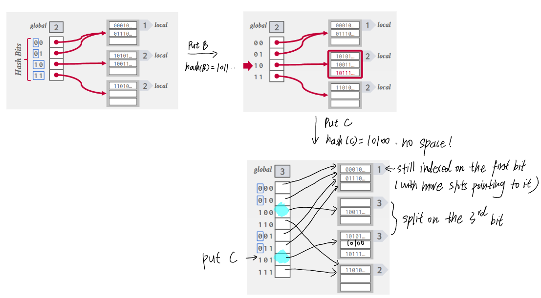
6.2. Extendible hashing
- Improve chained hashing to avoid letting chains grow forever.
- Allow multiple slot locations in the hash table to point to the same chain.
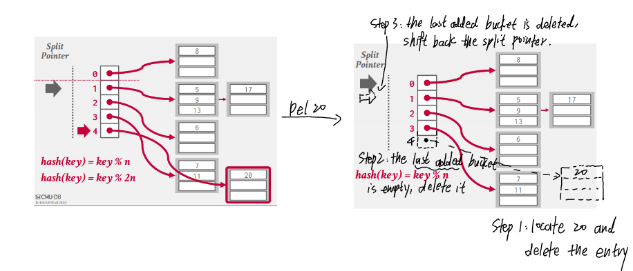
6.3. Linear hashing
- Maintains a split pointer to keep track of next bucket to split, even if the pointed bucket is not overflowed.
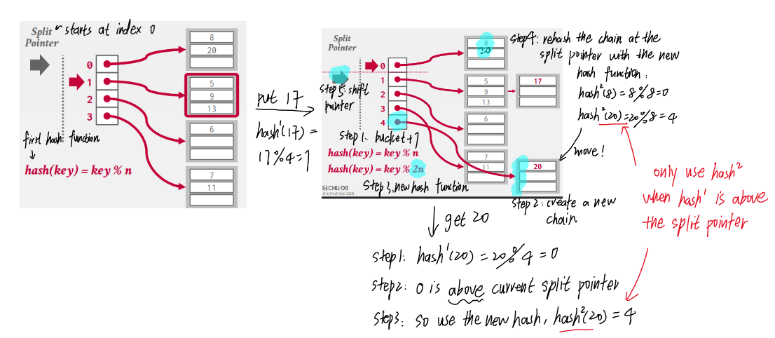
- There are always only 2 hash functions: \((key\ mod\ n)\) and \((key\ mod\ 2n)\) where \(n\) is the length of buckets when the split pointer is at the index 0 (i.e., the bucket length at any time is \(n + index(sp)\)).
- Why does \(k\ mod\ 2n < n + sp\) hold?
- A key is only mod by \(2n\) if the result of \((k\ mod\ n)\) is above the split pointer, i.e., \(0 \leq k\ mod\ n < sp)\).
- Let \(r = k\ mod\ n\), then \(k = pn + r\) and \(0 \leq r < sp\).
- Let \(r' = k\ mod\ 2n\), then \(k = q(2n) + r'\).
- If \(p = 2m\), then we also have \(k = m(2n) + r = q(2n) + r'\), in this case \(0 \leq r = r' < sp\).
- If \(p = 2m + 1\), then we have \(k = m(2n) + r + n = q(2n) + r'\), in this case \(n \leq r' = n + r < n + sp\).